Rheology

Learning Objectives

At the end of this lecture, student will be able to

• Explain the concept of rheology and viscosity in pharmacy
• Discuss the applications of viscosity, kinematic and dynamic viscosity in pharmaceuticals
• Discuss Newton’s law of flow and its relation to viscosity
• Discuss various factors influencing viscosity
• Explain the types of flow of pharmaceutical liquids
• Discuss the concepts of Newtonian and non-Newtonian flow
• Explain Plastic and Pseudoplastic systems of fluid with examples
• Discuss Shear thinning and Shear thickening systems
• Explain the concept of dilatant systems
• Discuss the reasons for dilatancy
• Describe the characters of dilatancy
• Explain thixotropy and its applications in pharmacy
• Explain the concept of single point and multi point viscometers
• Explain the method of determination of viscosity by various types of viscometers
• Discuss the advantages and disadvantages of viscometers
• Expl1ain the concept of thixotropy in pharmaceuticals
• Explain the Rheopectic flow behaviour of different liquids
• Describe the physical and chemical factors affecting rheological
• Discuss the pharmaceutical applications of rheology

Rheology

• Rheo – to flow
• Logos – science
• Rheology is the study of the flow and deformation of matter under stress.
• It is the study of the flow of materials that behave in an interesting or unusual manner

Rheogram:

• The plot between the shearing stress and rate of shear.

Definition of Rheology

• The branch of physics, which deals with deformation and flow of matter.
• Rheology governs the circulation of blood & lymph through capillaries and large vessels, flow of mucus, bending of bones, stretching of cartilage, and contraction of muscles.
• Fluidity of solutions to be injected with hypodermic syringes or infused intravenously, flexibility of tubing used in catheters, extensibility of gut.

Importance of Rheology

• Formulation of medicinal and cosmetic creams, pastes and lotions.
• Formulation of emulsions, suspensions, suppositories, and tablet coating.
• Fluidity of solutions for injection.
• In mixing and flow of materials, their packaging into the containers, their removal prior to use, the pouring from the bottle.
• Extrusion of a paste from a tube.
• Passage of the liquid to a syringe needle.
• Can affect the patient’s acceptability of the product, physical stability, biologic availability, absorption rate of drugs in the GIT
• Influence the choice of processing equipments in the pharmaceutical system.

From the rheological viewpoint systems are:

• Solid if they preserve shape & volume.
• Liquid if they preserve their volume.
• Gaseous if neither shape nor volume remains constant when forces are applied to them.

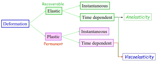
Mechanical Behaviour

• Elasticity Recoverable deformation
• Plasticity Permanent deformation
• Fracture Propagation of cracks in a material
• Fatigue Oscillatory loading
• Creep Elongation at constant load at High temperatures

Dynamic viscosity

• The unit of dynamic viscosity η is the “Pascal ⋅ second” [Pa⋅s].

• The unit “milli-Pascal ⋅ second” [mPa⋅s] is also often used.

– 1 Pa ⋅ s = 1000 mPa⋅s

• The previously used units of “centiPoise” [cP] for the dynamic viscosity η are interchangeable with [mPa⋅s].

– 1 mPa⋅s = 1 cP

Typical viscosity values at 20°C [mPa⋅s]

Kinematic viscosity

• When Newtonian liquids are tested by means of some capillary viscometers, viscosity is determined in units of kinematic viscosity υ.

• The force of gravity acts as the force driving the liquid sample through the capillary.

• The density of the sample is additional parameter.

• Kinematic viscosity υ and dynamic viscosity η are linked.

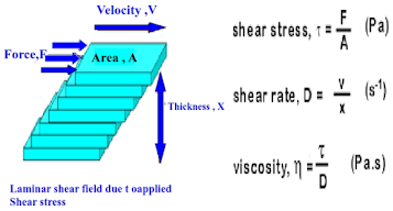
NEWTONS LAW

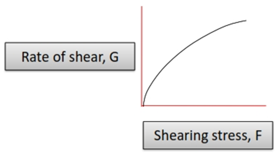
• According to Newtons law “higher the viscosity of a liquid, the greater is the force per unit area (shearing stress F) required to produce a certain rate of shear (G)”.

• Rate of shear α shearing stress

F= ῃ G

Where

F= F’/ A

G= dv/ dr

ῃ= viscosity

Newton Law of Flow

• Laminar or Stream line: The bottom layer is considered to be fixed in place. If the top plane of liquid is moved at a constant velocity, each lower layer will move with a velocity ∞ to its distance from the stationary layer.

• Velocity gradient or rate of shear, dv / dr.

• The rate of shear indicates how fast the liquid flows when a shear stress is applied to it. Its unit is sec-1.

• The force per unit area (F’/A) required to bring about flow is called the shearing stress and its unit is dyne/cm2.

F’/A = η dv / dr (1)

Where η is the viscosity.

Equation (1) is frequently written as:

η = F/G   (2)

Where F = F’/A   &
G = dv/dr.

For Newtonian System is shown in the figure. A straight line passing through the origin is obtained.

Viscosity

• It is defined as resistance to the flow.

• Viscosity (h) is the resistance of a fluid material to flow under stress. The higher the viscosity, the greater the resistance

• ῃ is the coefficient of viscosity. And is calculated as

ῃ=F/ G

Where F= Shearing stress

G= Rate of shear

• Unit of viscosity is Poise or dyne.sec/cm2.

Units of Absolute Viscosity

The Poise (p), is the shearing force required to produce a velocity of 1 cm/sec. between two parallel planes of liquid each 1 cm2 in area & separated by a distance of 1 cm.

• The Centipois (cp), 1 cp = 0.01 poise.

• Fluidity (f) is the reciprocal of viscosity:

(f)   =   1/η
(3)

• Kinematic viscosity: is the absolute viscosity divided by the density of the liquid

η/ρ            (4)

The units of kinematic viscosity are the stoke (s) & the centistoke (cs).

Effect of Temperature on Viscosity

• Viscosity of a gas increases with the increase of temperature.

• Viscosity of liquid decreases as the temperature is raised & the fluidity of a liquid, increases with temperature.

FACTORS AFFECTING VISCOSITY

• Intrinsic Factors:

a. Molecular weight – Heavier the molecular weight, higher the viscosity

b. Shape of particles; Large and irregularly shaped particles will be more viscous spheroid colloids is less viscous than linear colloids, as the latter tend to form a network within the dispersion medium.

c. Higher the intermolecular interactions, viscosity will increase

• Extrinsic factors:

a. Pressure – Increase in pressure increases

• Added substances influences viscosity. Eg. Nonelectrolytes like sucrose glycerin increases viscosity, storng electrolytes like metal and ammonium ions decerases visocity.

• Temperature; inverse relationship

Types of Flow

The choice depends on whether or not their flow properties are in accordance to Newton’s law of flow.

1. Newtonian                                    

2. Non – Newtonian

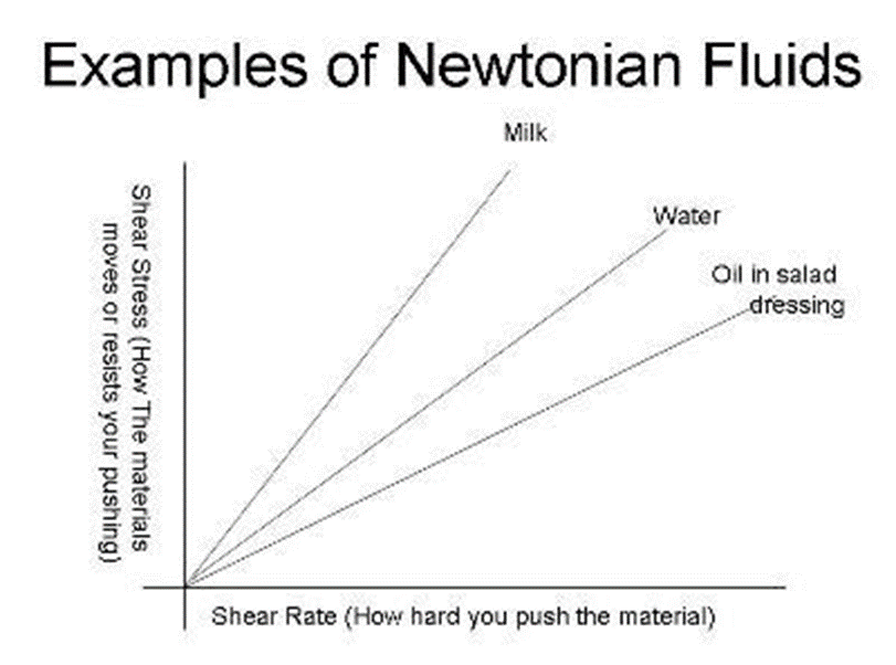
Newtonian flow

• A Newtonian fluid (named for Isaac Newton) is a fluid whose stress versus rate of shear curve is linear and passes through the origin. The constant of proportionality is known as the viscosity.

• Examples:

1. Water

2. Chloroform

3. Castor oil

4. Ethyl Alcohol

• Shows constant viscosity regardless of shear rates applied at a given temperature.

• Exhibit true viscosity

• Obeys newtons law

• Ex: water, dilute suspensions,

• True solutions.

• Curve pass through origin

• Slope gives co-efficient of viscosity

Non-Newtonian flow

• A non-Newtonian flow is defined as one for which the relation between F and S is not linear.

• In other words when the shear rate is varied, the shear stress is not varied in the same proportion. The viscosity of such a system thus varies as the shearing stress varies.

• It can be seen in liquids and in solid heterogeneous dispersions such as emulsions, suspensions, colloids and ointments.

Non newtonian systems

Three classes:

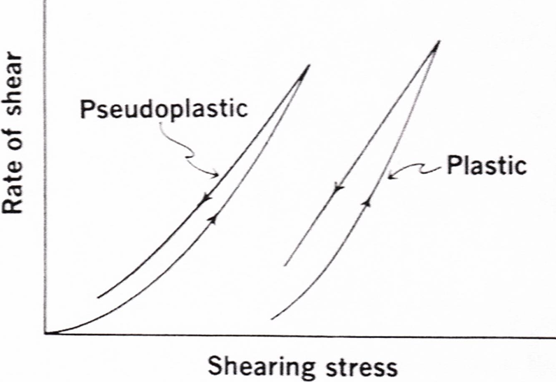
• Plastic flow

• Pseudoplastic Flow

• Dilatent Flow

PLASTIC FLOW

• In which curve does not pass through the origin, the substance behaves initially elastic body and it fails to flow when less amount of stress is applied.

• As increase the stress, leads to non-linear increase in shear rate but after that curve is linear.

• The linear portion extrapolated intersects the x axis at the point called as yield value.

• The plastic flow curve it intersects the shearing stress axis (or will if the straight part of the curve is extrapolated to the axis) at a particular point referred to as yield value. (f)

• Plastic flow shows Newtonian flow above the yield value.

• The curve represents plastic flow, such materials are called as Bingham bodies.

• Bingham bodies does not flow until the shearing stress is corresponding to yield value exceeded. A Bingham body does not begin to flow until a shearing stress, corresponding to the yield value, is exceeded.

• The reciprocal of mobility is Plastic viscosity

• EXAMPLES: ZnO in mineral oil, certain pastes, paints and ointments.

• The slope of the rheogram = mobility, (fluidity in Newtonian systems).

• Its reciprocal is known as the plastic viscosity.

U = (F-f) / G

Where,

f = Yield value

F = Shearing stress

G = Rate of shear

U = Plastic viscosity

• Plastic flow is associated with the presence of flocculated particles in concentrated suspensions.

• Yield value represents the stress required to break the inter-particle contracts so that particles behaves individually.

• The yield value is present due to contacts between adjacent particles (brought about by Van der Waal’s forces).

• Consequently, the yield value is an indication of the force of flocculation, the more flocculated the suspension, the higher will be the yield value.

• Frictional forces between moving particles can also contribute to the yield value.

• Once the yield value has been exceeded, any increase in shearing stress (i.e. F-f) brings about a directly proportional increase in G, the rate of shear.

• Aplastic system resembles a Newtonian system at shear stresses > the yield value.

• Plastic flow explained by flocculated particles in concentrated suspensions, ointments, pastes and gels.

Pseudo plastic flow

• Many Pharmaceutical products liquid dispersion of natural and synthetic gums shows pseudo plastic flow.

• eg. Tragacanth in water, Sodium Alginate in water, Methyl cellulose in water

• With increase in the shearing stress the disarranged molecules orient themselves in the direction of flow, thus reducing friction and allows a greater rate of shear at each shearing stress.

• Some of the solvent associated will be released resulting in decreased viscosity.

• This type of flow behavior is also called as shear thinning system.

• In which curve is passing from origin (Zero shear stress), so no yield value is obtained.

• As shear stress increases, shear rate increases but not linear.

• Pseudo plastic flow can be explained by Long chain molecules of polymer.

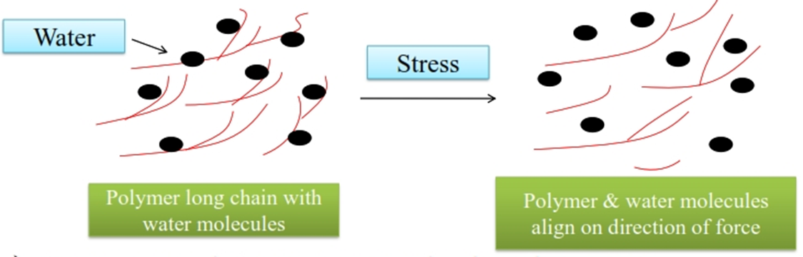
• In storage condition, arrange randomly in dispersion

• On applying F/A, shearing stress molecules (water & polymer) arrange long axis in the direction of force applied.

• This stress reduces internal resistance & solvent molecules released form polymer molecules.

• Then reduce the concentration and size of molecules with decrease in viscosity.

• The exponential equation shows this flow

FN = η G

N = no. of given exponent

η = Viscosity coefficient

• In case of pseudo plastic flow, N > 1.

i.e. More N >1, the greater pseudo plastic flow of material.

• If N = 1, the flow is Newtonian.

Taking Log on both sides,

N log F = log η + log G

On rearrangement, we get

log G = N log F – log η

This equation gives straight line,

• As the shearing stress á the normally disarranged molecules begin to align their long axes in the direction of flow. This orientation reduces the internal resistance of the material and allows a greater rate of shear at each successive shearing stress.

• In addition, some of the solvent associated with the molecules may be released, resulting in an effective lowering of the concentration and size of dispersed molecules.

• An equilibrium exists between the shear induced changes and random coiling tendency caused by Brownian motion which entraps water inside the coils. The rate of entanglement and randomization by Brownian motion is constant, while the rate of disentanglement and alignment increases with increasing shear stress.

• The viscosity diminishes as the shear is increased, so they are known as “shear thinning systems”.

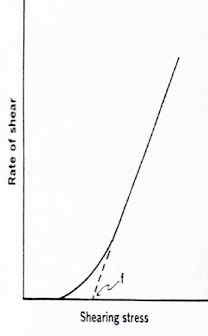
Dilatant flow

• Certain suspensions with high % of dispersed solids shows an increase in resistance to flow with increasing rates of shear, such system increase in volume when sheared, such system called as dilatant flow.

• Also, called as “Shear thickening system” i.e. when stress is removed, dilatant system return to its original position

Graph for dilatant flow is like this

• In which curve is passing from origin (Zero shear stress), so no yield value is Obtained.

• Non-linear increase in rate of shear.

• Increase resistance to flow on increase rate of shear

• In which, particles are closely packed with less voids spaces, also amount of vehicle is sufficient to fill the void volume.

• This leads particles to move relative to one another at low rate of shear.

• So therefore, dilatant suspension can be poured from bottle boz in these condition it is fluid.

• When stress is increased, the particles shows the open packing and bulk of system (void volume is increase) is increased.

• But the amount of vehicle is insufficient to fill this void space.

• Thus particles are not wetted or lubricated and develop resistance to flow.

• Finally system show the paste like consistency.

• Because of this type of behavior, the dilatant suspension can be process by high speed mixers, blenders or mills.

The exponential equation shows this flow

F^N = η G

N = no. of given exponent

η = Viscosity coefficient

In which N < 1, and decrease as the dilatancy Increase

If N = 1, the system is Newtonian flow

Reasons for Dilatency

• At rest particles are closely packed with minimal inter-particle volume (void), so the amount of vehicle is enough to fill in voids and permits particles to move at low rate of shear.

• Increase shear stress, the bulk of the system expand (dilate), and the particles take an open form of packing.

• The vehicle becomes insufficient to fill the voids between particles. Accordingly, particles are no longer completely wetted (lubricated) by the vehicle.

• Finally, the suspension will set up as a firm paste.

• This process is reversible.

Characters of Dilatant System

Resting	Sheared
Closed pack particles	Open packed particles
Minimum void volume	Increased void volume
Insufficient vehicle	Sufficient

 

• It describes pseudo-plastic liquids which additionally feature a yield point.

• They are mostly dispersions which at rest can build up an intermolecular/interparticle network of binding forces (polar forces, van der Waals forces, etc.).

• These forces restrict positional change of volume elements and give the substance a solid character with an infinitely high viscosity.

• Forces acting from outside, if smaller than those forming the network, will deform the shape of this solid substance elastically.

• Only when the outside forces are strong enough to overcome the network forces — surpass the threshold shear stress called the “yield point” — does the network collapse.

• Volume elements can now change position irreversibly: the solid turns into a flowing liquid.

• Typical substances showing yield points include oil well drilling muds, greases, lipstick masses, toothpastes and natural rubber polymers.

• Plastic liquids have flow curves which intercept the ordinate not at the origin, but at the yield point level of τ0.

Time Dependent Behaviour

Newtonian systems

• If the rate of shear was reduced once the desired maximum rate had been reached, the down curve would be identical with & superimposed on the up-curve.

Non Newtonian systems

With shear-thinning systems (i.e., plastic & pseudoplastic), the down – curve is frequently displaced to the left of the up-curve. This means that the material has a lower consistency at any one of shear on the down-curve than it had one rate of shear on the down-curve than it had on the up curve.

Pharmaceutical and Biological Applications of Rheology

1- Prolongation of Drug Action

• The rate of absorption of an ordinary suspension differs from thixotropic suspension.

• Example: procaine penicillin G, a form of penicillin, of relatively low water solubility. Aqueous suspensions containing between 40 and 70% w/v of milled or micronized procaine penicillin G + small amount of sodium citrate & polysorbate 80 are thixotropic pastes & are of depot effect when injected intramuscularly.

2- Effect on Drug Absorption

• The viscosity of creams and lotions may affect the rate of absorption of the products by the skin.

• A greater release of active ingredients is generally possible from the softer, less viscous bases.

• The viscosity of semi-solid products may affect absorption of these topical products due to the effect of viscosity on the rate of diffusion of the active ingredients.

(3) Thixotropy in Suspension and Emulsion Formulation

• Thixotropy is useful in the formulation of pharmaceutical suspensions and emulsions. They must be poured easily from containers (low viscosity)

• Disadvantages of Low viscosity:

– Rapid settling of solid particles in suspensions and rapid creaming of emulsions.

– Solid particles, which have settled out stick together, producing sediment difficult to redisperse (“caking or claying”).

– Creaming in emulsions is a first step towards coalescence. (Break down of emulsion)

• A thixotropic agent such as sodium bentonite magma, colloidal silicon dioxide, is incorporated into the suspensions or emulsions to confer a high apparent viscosity or even a yield value.

• At rest:

• High viscosities retard sedimentation & creaming.

• Yield values prevent them altogether; since there is no flow below the yield stress, the apparent viscosity at low shear becomes
infinite

• Pouring the suspension or emulsion from its container:

• Shaking at shear stresses above the yield value

• The agitation breaks down the thixotropic structure so reducing the yield value to zero & lowering the apparent viscosity. This facilitates pouring.

• Back on the shelf, the viscosity slowly increases again and the yield value is restored as Brownian motion rebuilds the house-of- cards structure of bentonite.

Determination of rheologic (flow) properties

Selection of viscometer

Type	Single point Viscometer	Multi point viscometer
Example	Ostwald viscometer Falling sphere viscometer	Cup and bob viscometer Cone and plate viscometer
Principle	Stress α rate of shear Equipment works at Single rate of shear	Viscosity det. at several rates of shear to get consistency curves
Application	Newtonian flow	non -Newtonian flow Newtonian flow

Single point viscometers

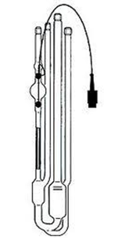
Ostwald viscometer (Capillary)

• The Ostwald viscometer is used to determine the viscosity of Newtonian fluid.

• The viscosity of Newtonian fluid is determined by measuring time required for the fluid to pass between two marks.

Principle: When a liquid flows by gravity, the time required for the liquid to pass between two marks ( A & B) through the vertical capillary tube. the time of flow of the liquid under test is compared with time required for a liquid of known viscosity (Water).

• Therefore, the viscosity of unknown liquid (η1) can be determined by using following equation:

ρ_1t1

 η ₁ = ——-η₂ Eq.1

ρ₂t₂

Where,

ρ1 = density of unknown liquid

ρ2 = density of known liquid

t1 = time of flow for unknown liquid

t2 = time of flow for known liquid

η2 = viscosity of known liquid

Eq. 1 is based on the Poiseuille’s law express the following relationship for the flow of l

η = П r2 t Δ P / 8 l V                                Eq:2

Where,

r = radius of capillary, t = time of flow, Δ P = pressure head dyne/cm2 ,

l = length of capillary cm, V = volume of liquid flowing, cm3

For a given Ostwald viscometers, the r, V and l are combine into constant (K), then eq. 2 can be written as,

η = KtΔP                           Eq.3

In which,

• The pressure head ΔP ( shear stress) depends on the density of liquid being measured, acceleration due to gravity (g) and difference in heights of liquid in viscometers.

• Acceleration of gravity is constant, & if the levels in capillary are kept constant for all liquids,

• If these constants are incorporate into the eq. 3 then, viscosity of liquids may be expressed as:

η1 = K’ t1 ρ1           eq. 4

η2 = K’ t2 ρ2          eq. 5

• On division of eq. 4 and 5 gives the eq .1, which is given in the principle,

ρ_1t1

η ₁ =——-η₂ Eq.6

ρ₂t₂

• Equation.6, may be used to determine the relative an absolute viscosity of liquid.

• This viscometer, gives only mean value of viscosity because one value of pressure head is possible.

• Ostwald viscometer is used for highly viscous fluid i.e. Methyl cellulose dispersions

Applications of Ostwald Viscometer 

• It is used in the formulation and evaluation of Pharmaceutical dispersions system such as colloids, suspensions, emulsions etc.

• It is official in IP for the evaluation of liquid paraffin, light liquid paraffin and dextran 40 injection.

Falling sphere viscometers

• It is called as Hoeppler falling sphere viscometers.

Principle: A glass or ball rolls down in vertical glass tube containing the test liquid at a known constant temprature. The rate at which the ball of particular density and diameter falls is an inverse function of viscosity of sample.

Construction:

• Glass tube position vertically.

• Constant temprature jacket with water circulation around glass tube

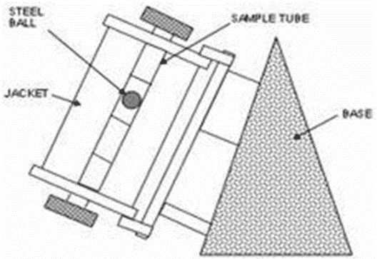
Working: A glass or steel ball is dropped into the liquid & allowed to reach equilibrium with temprature of outer jacket. The tube with jacket is then inverted so that, ball at top of the inner glass tube. the time taken by the ball to fall between two marks is measured, repeated process for several times to get concurrent results. For better results select ball which takes NLT 30 sec. to fall between two marks.

η = t ( Sb – Sf ) B

Where,

t = time in sec.for ball to fall between two marks

Sb & Sf = Specific gravities of ball and fluid under examination.

B = Constant for particular ball.

Multi point viscometers (Rotational)

Cup and Bob

• Various instruments are available, differ mainly whether torque results from rotation of cup or bob.

• Couette type viscometers: Cup is rotated, the viscous drag on the bob due to sample causes to turn. The torque is proportional to viscosity of sample

Ex. McMichael viscometer

• Searle type viscometers: Bob is rotated, the torque resulting from the viscous drag of the system under examination is measured by spring or sensor in the drive to the bob.

Ex. Stormer viscometer

Working: The test sample is place in space between cup and bob & allow to reach temperature equilibrium. A weight is place in hanger and record the time to make 100 rotation by bob, convert this data to rpm. This value represent the shear rate, same procedure repeated by increasing weight.

So then plotted the rheogram rpm Vs weights the rpm values converted to actual rate of shear and weight converted into units of shear stress, dy/cm2 by using appropriate constants.

Mathematical treatment:

For, rotational viscometers, the relationship can be expressed as,

η = Kv w/v

Where

v, rpm generated by

Weight w, in gm

Kv is obtained by analyzing material of known viscosity in poise.

Plug Flow

• Sample is placed between cup and bob

• During motion, when bob rotates, amount of stress exerted near the wall of bob is high compared to stress at inner wall of cup

• Stress will be varying at different areas

• So this may not represent the stress of entire sample

• This can be minimized by

– Using large bob

– Increasing RPM of bob

• Plug flow is undesirable for flow of dispersion systems but suitable for flow of paste

Cone and plate viscometer (Rotational viscometer)

Principle: The sample is placed on at the center of the plate, which is raised into the position under the cone. The cone is driven by variable speed motor and sample is sheared in the narrow gap between stationary plate and rotate Rate of shear in rpm is increased & decrease by selector dial and viscous traction or torque (shearing stress) produced on the cone.

• The sample is placed at the center of the plate which is then raised into position under the cone.

• The cone is driven by a variable speed motor & the sample is sheared in the narrow gap between the stationary plate and the rotating cone.

• The rate of shear in rev. /min. is increased & decreased by a selector dial & the torque (shearing stress) produced on the cone is read on the indicator scale.

• A plot of rpm or rate of shear versus scale reading or shearing stress may be plotted

C is an instrumental constant.

T is torque reading.

V is speed in revolution / minute.

η = C T / V

U = C   (T – T _f) / V

f = T f   x C f                   Cf is constant  Plastic materials

Advantages

• The rate of shear is constant throughout the entire sample being sheared. As a result, any change in plug flow is avoided.

• Time saved in cleaning & filling.

• Temperature stabilization of the sample during a run.

• The cone and plate viscometer requires a sample volume of 0.1 to 0.2 ml. This instrument could be used for the rheological evaluation of some pharmaceutical semisolids.

Brookefield Viscometer

Viscosity for Newtonian system can be estimated by,

Where,

η = C T/V                eq.1

C = Instrument constant,

T = Torque reading & V = Speed of the cone (rpm)

Plastic viscosity determined by,

U = Cf   T – Tf / v              eq.2

Yield value (f) = Cf × Tf

Tf = Torque at shearing stress axis (extrapolate from linear portion of curve).

Cf = Instrument constant

THIXOTROPHY

Definition

• It is a isothermal and comparatively slow recovery, on standing of a material which lost its consistency through shearing.”

• Thixotropy is only applied to shear-thinning systems. This indicates a breakdown of structure (shear-thinning), which does not reform immediately when the stress is removed or reduced.

At rest – Gel structure

Asymmetric particles, many points of contact, network structure, small Low viscosity & rigid structure.

â Shearing stress

Sol State

Breakdown of structure, flow starts, particles are aligned and Particle collisions, contacts are more,transform to sol (shear thinning)

â Removal of Shearing stress

Gel structure

Rebuild of the gel structure by brownian motion, flocs contacts break,

Individual particles, low consistency, (time is not defined)

• Thixotropic systems usually contain asymmetric particles which, possess numerous points of contact & set up a loose three-dimensional network.

• At rest, this structure confers some degree of rigidity on the system & it resembles a gel.

• As shear is applied & flow starts, this structure begins to break down. Points of contact are disrupted & the particles become aligned.

• The material undergoes a gel-to-sol transformation & exhibits shear thinning. Eg. aqueous dispersion of 8% w /w sodium

• Upon removal of the stress, the structure starts to reform. This process is not immediate.

• It is a progressive restoration of consistency as the asymmetric particles come into contact with each other by undergoing random brownian movement.

• The rheograms obtained with thixotropic materials are dependent on:

1- The rate at which shear is increased or decreased.

2- The time for which a sample is subjected to any one rate of shear.

• The Figure describes thixotropy in graphical form.
• In the flow curve the “up-curve” is no longer directly underneath the “down-curve”.
• The hysteresis now encountered between these two curves surrounds an area “A” that defines the magnitude of this property called thixotropy.
• This area has the dimension of “energy” related to the volume of the sample sheared which indicates that energy is required to break down the thixotropic structure

The distinction between a thixotropic fluid and a shear thinning fluid:

• A thixotropic fluid displays a decrease in viscosity over time at a constant shear rate.
• A shear thinning fluid displays decreasing viscosity with increasing shear rate.
• Some fluids are anti-thixotropic: constant shear stress for a time causes an increase in viscosity or even solidification. Constant shear stress can be applied by shaking or mixing.

Rheopexy

• It is a phenomenon in which a sol transforms to a gel more readily rather than keeping a sol at rest.
• Shaking or low rate of shear is sufficient to transform a sol into gel.
• At equilibrium the system is in gel state, while antithixotrophy exhibits sol form

An increase in apparent viscosity with time under constant shear rate or shear stress, followed by a gradual recovery when the stress or shear rate is removed.

Bulges

• The curve produces a Hystersis loop with a characteristic bulge in the up-curve
• This is due to the crystalline plates that form a “Cage like Structure” that causes swelling in the formulation
• Eg: Bentonite Magma

Spur

• This is a rheogram wherein the bulged curve may develop into a
• “spur like protrusion”
• Spur value represents a sharp point of structural breakdown at a low shear rate in the up-curve
• But spur value will be missed out if shear stress at low shear rate are not recorded properly
• Eg. Procaine Penicillin gel

Negative Thixotrophy

• Also called as anti thixotrophy
• It represents increase in consistency of the down curve. Eg. Magnesia Magma
• Magnesia magma exhibits enhanced resistance to flow with increased time of shear compared to resting state
• When magma is sheared alternatively with increasing and decreasing rate of shear, magma thickens
• As this continues, extent of thickening decreases gradually and reaches equilibrium and there will be no change in the consistency curves on further cycles of shear rate
• Its molecular mechanism is explained as following:

At rest – On storage –  Gel structure

Low viscosity-small flocs- individual particles are in large number

â  Shearing stress

Equilibrium – Sol state

Particle collisions, contacts are more, large flocs are in small number

High consistency

â  Removal of Shearing stress

Set Aside

Flocs contacts break individual particles – Low consistency

Measurement of Thixotrophy

Method 1:

1. In a thixotrophic system the hysteresis loop is formed by the up and down curves of the rheogram
2. The area of hysteresis loop represents thixotropic breakdown c. It can be obtained with the help of planimeter

Method 2:

1. The nature of rheogram largely depends on the rate at which shear is increased or decreased
2. Suppose shear rate is increased at a constant rate on the system upto point ‘b’ and then decreased
3. when the results are plotted ’abe’ rheogram is obtained. If the shear rate is maintained at ‘b’ for time ‘t1’ secs and then decreased, ‘abce’
4. Similarly at point ‘b’ if the shear rate is maintained for time ‘t2’ seconds and then decreased, ‘abde’ curve is obtained
5. Structural breakdown w.r.t time at constant rate of shear gives the rheogram
6. Based on these rheograms, Thixotropic Co-efficient “B” is calculated by the equation

       (U1-U2)

B=  —————

     ln(t2/t1)

U1 and U2 = Plastic viscosities of two down curves

1. Thixotropic Co-efficient “B” represents the rate of break down

Method 3:

1. The system is subjected to different rates of shear (say V1 and V2) and the rheogram is obtained, which shows TWO hysteresis loops.
2. The Thixotropic Co-efficient “M” is calculated by the equation

         2(U1-U2)

M  =  —————-

          ln(V2Vt1)2

U1 and U2 = Plastic viscosities of two down curves having shear rates V1 and V2

1. Thixotropic Co-efficient “M” represents the loss in shearing stress per unit increase in shear rate

Applications:

• Thixotrophy is desirable in emulsions, suspensions and creams
• Greater the thixotrophy, higher the physical stability of suspension
• Degree of thixotrophy is related to specific surface Eg: Procaine Penicillin G parentreal suspension – while injecting structural break down takes place and product pass through hypodermic needle – after injection original structure of gel will rebuilt – this leads to Depot of penicillin at the site of injection in the muscle from which it is slowly released providing sustained action

Factors Affecting Rheological Properties in Pharmaceuticals

Chemical Factors

(a) Degree of Polymerization

• Suspending agents, and emulsion stabilizers act in low concentrations to produce viscous solutions (high molecular weight).
• Lower concentrations of the high molecular weight grades of synthetic & modified natural gums are used to obtain the desired viscosity.

(b) Extent of Polymer Hydration

• In hydrophilic polymer solution the molecules are completely surrounded by immobilized water molecules forming a solvent layer. Such hydration of hydrophilic polymers gives rise to an increased viscosity.
• The solvate layer is strongly bound to the macromolecule viscosity will be insensitive to pH changes or low concentrations of electrolytes.
• Loose solvate around the macromolecules, pH & electrolytes will produce

(c) Impurities, Trace Ions and Electrolytes

• Changing the viscosity of natural polymers, e.g. in sodium alginate solution, the viscosityá to the gelling point â the formation of calcium alginate.
• Atáconcentrations, electrolytes do not change the viscosity of natural colloids in aqueous solution.
• Concentrations, the salts compete for the adsorbed water molecules, surrounding the hydrated polymer, due to the affinity of the salt ions for water.
• As the polymer molecules become dehydrated, their dispersions decrease in viscosity & precipitation occurs

(d) Effect of pH

• Changes in pH greatly affect the viscosity & stability of the hydrophilic natural & synthetic gums.
• The natural gums usually have a relatively stable viscosity plateau extending over 5 or 4 pH units. Above and below this stable pH range viscosity decreases sharply.
• Sodium salts polymers are unstable in acid medium due to the separation of the acid form of the polymer, e.g. sodium alginate.

(E) Sequestering Agents and Buffers

• Sequestering agents have a stabilizing effect on viscosity in some polymer solutions, which are decomposed by traces of metals. Ex: Calcium ionsáthe viscosity of sodium alginate. Addition of sequestering agents i.e. EDTA or hexameta-phosphate will viscosity in sodium alginate solutions.

Physical Factors

(a) Aeration

• Aerated products usually result from high shear milling. Aerated samples are more viscous or have more viscous creamed layer than non-aerated samples.
• Some aerated emulsions will be less viscous & less stable than un-aerated samples due to concentration of the surfactant or emulsion stabilizer at the air liquid interface & thus deletion of the stabilizer at the oil – water interface.

De-aeration is done:

• Mechanically by roll milling, which squeezes out the air.
• Heat the aerated system.

(b) The Degree of Dispersion and Flocculation

• In concentrated suspensions of 3% solids & higher, a decrease in particle size of the solid phase, produce an increase in the viscosity of the system.
• This viscosity increase to immobilization of the vehicle with an increase in the fraction of the suspension volume effectively occupied by the solid.
• The addition of insoluble solids to a Newtonian vehicle non-Newtonian flow properties in system.
• The smaller the particle size of the dispersed solid phase, the lower the concentration of the solids required to produce non-newtonian flow

(c)  Light

• Various hydrocolloids in aqueous solutions are reported to be sensitive to light. These colloids include carbopol, sodium alginate & sodium carboxymethyl cellulose.
• To protect photosensitive hydrocolloids from decomposition:
• The use of light-resistant containers,
• Screening agents, antioxidants.

Summary

• Rheology is the study of the flow and deformation of matter under stress.
• It is the study of the flow of materials that behave in an interesting or unusual manner
• Rheogram is the plot between the shearing stress and rate of shear.
• Kinematic viscosity – When Newtonian liquids are tested by means of some capillary viscometers, viscosity is determined in units of kinematic viscosity υ.
• The force of gravity acts as the force driving the liquid sample through the capillary.
• According to Newtons law “higher the viscosity of a liquid, the greater is the force per unit area (shearing stress F) required to produce a certain rate of shear (G)”.
• Newtonian fluid is a fluid whose stress versus rate of shear curve is linear and passes through the origin. The constant of proportionality is known as the viscosity.
• A non-newtonian flow is defined as one for which the relation between F and S is not linear.
• When the shear rate is varied, the shear stress is not varied in the same proportion. The viscosity of such a system thus varies as the shearing stress varies.
• In pseudoplastic system, as the shearing stress is increased, disarranged molecules orient themselves to the direction of flow which reduces internal friction and resistance of the molecules and allows a greater rate of shear at each shear stress.
• Suspensions with high % of dispersed solids shows an increase in resistance to flow with increasing rates of shear, such system increase in volume when sheared, such system called as dilatant flow.
• Characters of dilatant system include both Resting and Sheared
• At rest particles are closely packed with minimal inter-particle volume (void), so the amount of vehicle is enough to fill in voids and permits particles to move at low rate of shear.
• Viscometers are used in the formulation and evaluation of Pharmaceutical dispersions system such as colloids, suspensions, emulsions etc. and they are official in IP for the evaluation of liquid paraffin, light liquid paraffin and dextran 40 injection.
• The rate of shear is constant throughout the entire sample being sheared. As a result, any change in plug flow is avoided.
• Time saved in cleaning & filling.
• Temperature stabilization of the sample during a run.
• Thixotropy is the property of some non- newtonian pseudoplastic fluids to show a time-dependent change in viscosity; the longer the fluid undergoes shear stress, the lower its viscosity.
• A thixotropic fluid is a fluid which takes a finite time to attain equilibrium viscosity when introduced to a step change in shear rate.
• Rheopexy is an increase in apparent viscosity with time under constant shear rate or shear stress, followed by a gradual recovery when the stress or shear rate is removed.

Also, Visit: Biotechnology Notes

B Pharma Notes

Enzyme Notes

Pharmacogonosy Notes for Pharma Students